As to investigate the influence of approximation schemes on
the description of protein structure and dynamics we first
analyze the temporal evolution of the rms deviations
![]() defined by eq. (8).
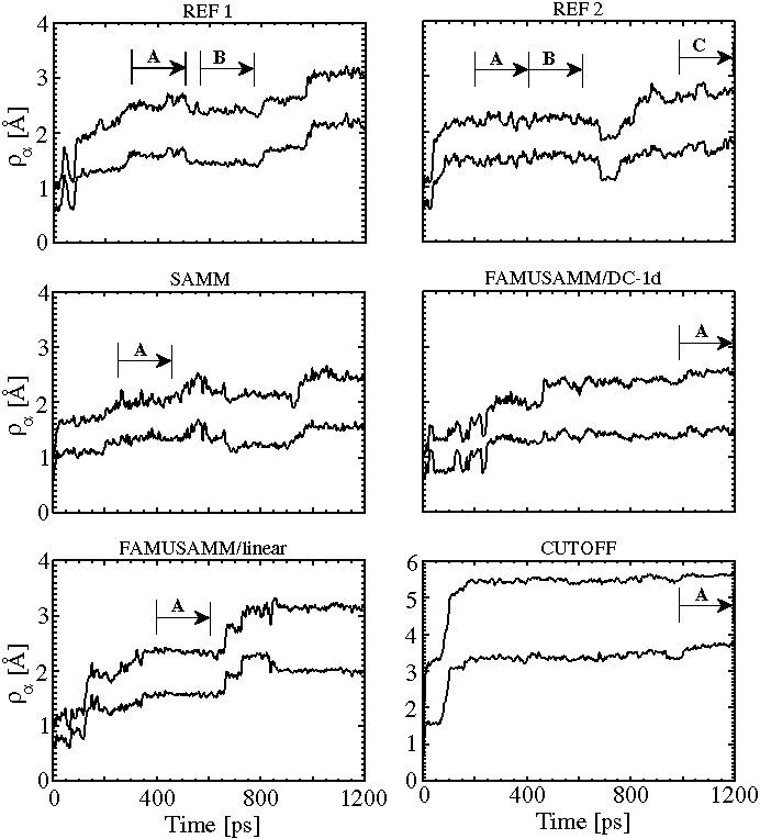
The graphs shown in Figure 5 have been
obtained from the various 1.2ns simulations of BPTI in vacuo.
The graphs represent smoothened versions of
defined by eq. (8).
The graphs shown in Figure 5 have been
obtained from the various 1.2ns simulations of BPTI in vacuo.
The graphs represent smoothened versions of
![]() obtained by taking local averages of 5ps width.
obtained by taking local averages of 5ps width.

Figure 5:
Temporal evolution of backbone rms deviations ![]() and side chain rms deviations
and side chain rms deviations ![]() for the two reference
simulations (REF1 and REF2) and the four approximation methods;
due to the flexibility of the side chains,
for the two reference
simulations (REF1 and REF2) and the four approximation methods;
due to the flexibility of the side chains, ![]() is always larger
than
is always larger
than ![]() ;
trajectory sections, which correspond to stable substates and are used
for later evaluation of the covariance matrices, are denoted by capital
letters; for explanation see text.
;
trajectory sections, which correspond to stable substates and are used
for later evaluation of the covariance matrices, are denoted by capital
letters; for explanation see text.
The rms deviations ![]() of the side chain atoms
are always larger than the rms deviations
of the side chain atoms
are always larger than the rms deviations ![]() of the backbone atoms,
since side chains are much more flexible than the protein
backbone.
As can also be seen in Figure 5, both
of the backbone atoms,
since side chains are much more flexible than the protein
backbone.
As can also be seen in Figure 5, both ![]() and
and
![]() increase with simulation time and generally exhibit a series
of jumps.
The first jump reflects the thermal fluctuations around the initial
structure, whereas later jumps, as shown by a closer inspection
of the associated structures (data not shown), arise from
conformational transitions.
increase with simulation time and generally exhibit a series
of jumps.
The first jump reflects the thermal fluctuations around the initial
structure, whereas later jumps, as shown by a closer inspection
of the associated structures (data not shown), arise from
conformational transitions.
Furthermore one recognizes from the top two plots in Figure 5
that the time development of the rms deviations
![]() distinctly differs for the two reference simulations
indicating that, indeed, the chaotic character of the system has led
to a complete decorrelation of the respective trajectories.
Yet the rms deviations resulting after 1.2ns are of similar
size and measure
distinctly differs for the two reference simulations
indicating that, indeed, the chaotic character of the system has led
to a complete decorrelation of the respective trajectories.
Yet the rms deviations resulting after 1.2ns are of similar
size and measure ![]() Å and
Å and
![]() Å
respectively.
Within the first 200ps our rms deviations agree well with those
obtained from other BPTI simulations in vacuo of up to 210ps
length [6, 2].
Å
respectively.
Within the first 200ps our rms deviations agree well with those
obtained from other BPTI simulations in vacuo of up to 210ps
length [6, 2].
Inspection of the subsequent three plots in Figure 5 shows
that for SAMM and FAMUSAMM the overall behavior of ![]() is similar
to that obtained for the two reference simulations.
All graphs exhibit jumps pointing towards conformational
transitions, and after 1.2ns the values of
is similar
to that obtained for the two reference simulations.
All graphs exhibit jumps pointing towards conformational
transitions, and after 1.2ns the values of ![]() are close
to those of the reference simulations.
are close
to those of the reference simulations.
In contrast, ![]() exhibits a qualitatively and quantitatively
different behavior for the cutoff simulation (lower right plot; note the
different scale).
Here one single and large conformational transition occurs after about
100ps, and subsequently conformational transitions are
suppressed
exhibits a qualitatively and quantitatively
different behavior for the cutoff simulation (lower right plot; note the
different scale).
Here one single and large conformational transition occurs after about
100ps, and subsequently conformational transitions are
suppressed .
As shown by an analysis of the proteins structure, the transition was
connected with a contraction upon which its overall size shrank
by about 5Å.
In summary, as monitored by ![]() , no essential differences
can be detected between the reference simulations, SAMM, and FAMUSAMM
simulations, whereas the cutoff simulation apparently describes
a different system.
, no essential differences
can be detected between the reference simulations, SAMM, and FAMUSAMM
simulations, whereas the cutoff simulation apparently describes
a different system.
We now turn to the investigation of dynamical correlations as described
by the covariance matrices ![]() defined in eq. (9).
As noted above, a comparison of such matrices requires that
the trajectories, from which the
defined in eq. (9).
As noted above, a comparison of such matrices requires that
the trajectories, from which the ![]() are calculated, refer to identical
or at least similar conformational substates of the protein.
Inspection of Figure 5 shows that one can identify a
couple of sections
within the trajectories of the simulations pointing to conformational
substates which are stable for at least 200ps.
These sections marked by
capital letters in Figure 5 were employed for evaluation
of associated covariance matrices.
are calculated, refer to identical
or at least similar conformational substates of the protein.
Inspection of Figure 5 shows that one can identify a
couple of sections
within the trajectories of the simulations pointing to conformational
substates which are stable for at least 200ps.
These sections marked by
capital letters in Figure 5 were employed for evaluation
of associated covariance matrices.
Differences between the covariance matrices calculated in this way can be due to various sources: (i) they may represent pure statistical fluctuations, (ii) they may reflect dynamical variations associated with the individual conformational substates, and (iii) they may be caused by the application of deviating computational methods.
In order to disentangle these sources we first provide an estimate for (i)
the size of statistical fluctuations.
For that purpose we chose the two consecutive 200ps sections of the
second reference trajectory, which are marked in Figure 5,
top right, as A and B.
As is indicated by the constancy of the ![]() in that period,
these sections refer to one and the same
conformational substate of BPTI.
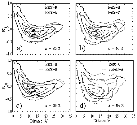
Figure 7(a) shows an overlay of the two covariance plots calculated
from the covariance matrices associated with these trajectory sections and
displays the value of the rms difference
in that period,
these sections refer to one and the same
conformational substate of BPTI.
Figure 7(a) shows an overlay of the two covariance plots calculated
from the covariance matrices associated with these trajectory sections and
displays the value of the rms difference ![]() between the
covariance matrices.
between the
covariance matrices.

Figure:
Covariance plots for comparison of BPTI dynamics within stable conformational
substates simulated by different methods (see text for explanation).
As one can see, the two plots are nearly identical.
They show strong positive correlations
between motions of neighboring atoms, which reflect the rigidity of the
covalently bonded structure.
At intermediate distances around ![]() Å anti-correlations dominate,
whereas correlations become positive again at distances larger than
Å anti-correlations dominate,
whereas correlations become positive again at distances larger than
![]() Å.
The rms deviation
Å.
The rms deviation ![]() of the two cross correlations is
of the two cross correlations is
![]() %.
Thus deviations
%.
Thus deviations ![]() have to be distinctly larger than that value,
and covariance plots have to exhibit much more pronounced differences
than those in Figure 7(a), as to exclude mere effects of statistical fluctuations
and to prove the existence of physical or algorithmic differences of the
simulated dynamics.
have to be distinctly larger than that value,
and covariance plots have to exhibit much more pronounced differences
than those in Figure 7(a), as to exclude mere effects of statistical fluctuations
and to prove the existence of physical or algorithmic differences of the
simulated dynamics.
A measure for the alteration of correlations of atomic motion, which is
induced by a conformational transition into a different substate [see
point (ii)], is provided by Figure 7(b).
This figure also shows covariance matrices extracted from the second reference
trajectory, but in contrast to Figure 7(a) trajectory sections referring to
different substates of BPTI are compared. Specifically, sections
B and C as
marked in Figure 5, top right, have been chosen for comparison.
In comparison to Figure 7(a), the covariance plots exhibit sizable differences,
and the rms deviation of cross correlations, measuring ![]() %,
is larger.
But note that, apparently, the conformational transition from state B to
state C has had little influence on the overall shape of the covariance plots.
%,
is larger.
But note that, apparently, the conformational transition from state B to
state C has had little influence on the overall shape of the covariance plots.
Similar conclusions may be drawn, if one considers Figure 7(c). This figure
compares covariance plots extracted from different trajectories calculated
with the same computational method, i.e., sections B of the first reference
simulation and section B of the second reference simulation
as marked in Figure 5, top plots.
These sections refer to slightly different
substates, which have been selected according to a criterion of maximal
structural similarity.
Consequently, the good match of the covariance plots in Figure 7(c) as
well as the low value of ![]() % indicates that closely
resembling structures exhibit similar dynamics.
% indicates that closely
resembling structures exhibit similar dynamics.
In order to finally pin down the range within which the rms deviations
![]() of cross correlations can vary upon conformational transitions
at a nanosecond time scale, we have additionally selected a whole set
of 200ps sections corresponding to stable substates from the two reference
trajectories.
We found that
of cross correlations can vary upon conformational transitions
at a nanosecond time scale, we have additionally selected a whole set
of 200ps sections corresponding to stable substates from the two reference
trajectories.
We found that ![]() never exceeded 70% and had a mean value
of 58%.
never exceeded 70% and had a mean value
of 58%.
We now are in a position to use our long time observables as to distinguish algorithmic artifacts from effects of statistical fluctuations and conformational transitions. For this purpose we will select from the trajectories calculated with the approximate methods 200ps sections with the following properties: (a) They should refer to stable substates, and (b) the structure of that substate should be as similar as possible to the structure of one of the substates sampled in one of the reference trajectories.
Figure 7(d) clearly indicates that the cutoff method is prone to algorithmic
artifacts concerning the description of dynamics. This conclusion is
validated in particular by the large value of 84% for the rms deviation
![]() , which, in contrast to the covariance plot, solely expresses
dynamical properties; note that the contour plots additionally display distance
information.
, which, in contrast to the covariance plot, solely expresses
dynamical properties; note that the contour plots additionally display distance
information.

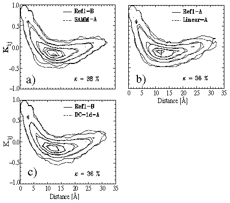
Figure: Further covariance plots for evaluation of our simulation methods.
Quite in contrast to the cutoff method all approximate methods, which
account for long range Coulomb interactions by structure-adapted multipole
expansions, show excellent performance in our test on dynamics.
This statement is proven by Figure 8 displaying the respective covariance
plots and the values of ![]() .
As monitored by the plots and by
.
As monitored by the plots and by ![]() , in all cases the substate
dynamics calculated by SAMM and FAMUSAMM resembles quite closely
to the dynamics of a similar substate sampled by the reference simulations.
The comparisons are as close as those between the sections B of the reference
simulations shown in Figure 7(c).
Furthermore we have also selected a set of 200ps sections
referring to arbitrary substates from the SAMM and FAMUSAMM trajectories
for comparison with substate sections from both reference simulations
using
, in all cases the substate
dynamics calculated by SAMM and FAMUSAMM resembles quite closely
to the dynamics of a similar substate sampled by the reference simulations.
The comparisons are as close as those between the sections B of the reference
simulations shown in Figure 7(c).
Furthermore we have also selected a set of 200ps sections
referring to arbitrary substates from the SAMM and FAMUSAMM trajectories
for comparison with substate sections from both reference simulations
using ![]() as the observable.
Like in the comparison among the reference sections noted
further above, no value larger than 70% was found for
as the observable.
Like in the comparison among the reference sections noted
further above, no value larger than 70% was found for ![]() .
As a consequence, concerning dynamics, no difference has been
detected between the exact evaluation of long range Coulomb forces
and our approximate methods.
.
As a consequence, concerning dynamics, no difference has been
detected between the exact evaluation of long range Coulomb forces
and our approximate methods.
Summarizing the results of our study on the accuracy of the various approximate MD algorithms we may state, that the FAMUSAMM/DC-1d algorithm (a) provides forces which are nearly as accurate as those obtained with SAMM, (b) entails only comparable little algorithmic noise, and (c) passes also our tests on the description of protein structure and dynamics with equally excellent results. In contrast, FAMUSAMM/linear is hampered by pronouncedly increased algorithmic noise, whereas the cutoff method exhibits unsatisfactory behavior in every respect. In view of these results we have discarded the linear multiple-time-step extrapolation scheme from further consideration within FAMUSAMM. It remains to be checked, to what extent the favorable algorithmic properties of FAMUSAMM are accompanied by a correspondingly favorable computation performance.