Another class of approximation schemes, the multiple-time-step methods [28, 29, 32, 16, 33]
, exploit complementary properties of protein electrostatics
for the same purpose; they take advantage of temporal
regularities.
The so-called distance class methods, in particular, are based on the
observation that forces originating from distant atoms fluctuate
more slowly than forces from atoms nearby (see Figure 3).
The slowly fluctuating forces may be evaluated less frequently than the fast
ones and may be extrapolated at the time steps in between.
Such extrapolation is required as the numerical integration of the dynamical
equations needs all forces at every integration time
step ![]() ,
which discretizes the simulation time
,
which discretizes the simulation time ![]() ,
where
,
where ![]() is the integration time step
size
is the integration time step
size .
.
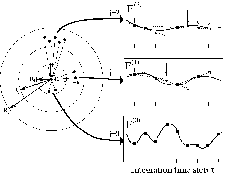
Figure: (left) Distance classes j=0,1,2,.., are defined for an atom (central dot)
by a set of radii ![]() generating a series of spherical shells;
(right) also shown is for each distance class the temporal evolution of the
total force
generating a series of spherical shells;
(right) also shown is for each distance class the temporal evolution of the
total force ![]() acting on the selected atom
originating from all atoms in the respective distance class;
along with the exact forces (solid line) and their exact values
(filled squares) also linear force extrapolations (dotted lines) and
resulting force estimates (empty squares) are depicted.
acting on the selected atom
originating from all atoms in the respective distance class;
along with the exact forces (solid line) and their exact values
(filled squares) also linear force extrapolations (dotted lines) and
resulting force estimates (empty squares) are depicted.
The left part of Figure 3 illustrates how distance
classes j can be defined by
a set of increasing radii ![]() .
The set of atoms
.
The set of atoms ![]() at positions
at positions
![]() satisfying
satisfying
![]() makes up the distance
class j of particle
l at position
makes up the distance
class j of particle
l at position
![]() .
As is also indicated in Figure 3 (right part),
for each particle l the sum of forces
.
As is also indicated in Figure 3 (right part),
for each particle l the sum of forces
![]() arising from
particles in distance class j is calculated explicitly every
arising from
particles in distance class j is calculated explicitly every
![]() -th
integration time step (filled squares).
Each of these time steps is called a macro integration step.
A common choice [16] is
-th
integration time step (filled squares).
Each of these time steps is called a macro integration step.
A common choice [16] is ![]() .
Correspondingly, the
.
Correspondingly, the ![]() elementary time steps within the cycle of a
macro integration step are called micro integration steps.
As sketched in Figure 3, at each step
elementary time steps within the cycle of a
macro integration step are called micro integration steps.
As sketched in Figure 3, at each step
![]() is estimated from two forces calculated
at previous macro integration steps by
is estimated from two forces calculated
at previous macro integration steps by
![]()
using appropriate extrapolation coefficients ![]() and
and
![]() .
The lower index of
.
The lower index of ![]() denotes the absolute integration time
step number and is expressed in terms of
the macro integration step
denotes the absolute integration time
step number and is expressed in terms of
the macro integration step ![]() and
the cyclic micro integration step
and
the cyclic micro integration step ![]() ;
;
![]() and
and
![]() are explicitly calculated at the macro integration
steps k and
k-1.
are explicitly calculated at the macro integration
steps k and
k-1.
The hierarchical extrapolation procedure sketched above is capable to save an enormous amount of computer time as it frequently avoids the most time consuming step, i.e., the exact evaluation of all interactions. Here computational speed is gained at the cost of an increased demand for memory: for each atom and each distance class two previous forces have to be kept in memory.
Various choices for the extrapolation coefficients
![]() and
and
![]() have been
discussed [16, 33, 37]; both the
linear extrapolation (illustrated in Figure 3) and
the so-called DC-1d algorithm have been found
promising [16]. Although the linear extrapolation defined by
have been
discussed [16, 33, 37]; both the
linear extrapolation (illustrated in Figure 3) and
the so-called DC-1d algorithm have been found
promising [16]. Although the linear extrapolation defined by
![]()
entails smaller discontinuities for the extrapolated forces than the
DC-1d algorithm, it leads to a larger energy transfer into a simulation
system by algorithmic noise [16].
The DC-1d scheme employs the coefficients
![]()
It is a priori not clear, whether the quoted properties of these extrapolation schemes will pertain, if they are combined with the SAMM procedure into our new FAMUSAMM scheme, which will be explained in the next section. Therefore, using test simulations we will subsequently check both extrapolation methods for their suitability within our combination method.